De-Urbanization of Surface Temperatures with the Landsat-Based “Built-Up” Dataset. Hentet fra Roy Spencer. Ph.D.
November 2nd, 2022
Overview
A relatively new global dataset of urbanization changes over the 40 year period 1975-2014 based upon Landsat data is used to determine the average effect urbanization has had on surface temperatures. A method is presented to compute the magnitude of the Urban Heat Island (UHI) effect on temperatures using the example of summertime 09 UTC (early morning) Integrated Surface Database (ISD) hourly data (mostly from airports) over the period 1973-2022 by comparing urbanization differences to temperature differences from closely-spaced weather stations. The results for the eastern U.S. lead to a 50-year warming trend 50% less than that from the official NOAA homogenized surface temperature dataset. It is likely that the daytime reductions in temperature trends will be less dramatic.
Background
Over the U.S., summertime warming in the official NOAA surface temperature record has been less than in all of the climate models used to guide national energy policy. That discrepancy could be even larger if spurious warming from increasing urbanization remains in surface temperature trends. While NOAA’s homogenization procedure has largely removed the trend differences between closely-spaced rural and urban stations, it is not clear whether the NOAA methodology actually removes increasing Urban Heat Island (UHI) effects since it’s possible it simply adjusts rural warming to match urban warming.
Anthony Watts has spearheaded a years-long effort to try to categorize how well-sited the USHCN network of temperature-monitoring stations is, and has found that the best-sited ones, on average, show temperature trends considerably lower than the official trends from NOAA. The well-sited thermometers are believed to have minimized the influence of local outbuildings, sidewalks, HVAC systems, parking lots, etc, on the trends. But economic growth, even in rural areas, can still lead to gradual spurious warming as the area outside the immediate vicinity of the thermometer undergoes growth. The issue is important enough that other methods of computing land-based temperature trends should be investigated. To that end, John Christy and I have been discussing ways to produce a new dataset of surface temperatures, with a largely independent set of weather stations and a very different data-adjustment philosophy.
Many readers here know I have been experimenting off an on over the years with U.S. surface thermometer data to try to determine how much U.S. warming trends have been affected by increasing urban influences. I have been trying to use datasets that can be applied globally, since it is impractical to visit and examine every weather observation site in the world. So far, I had been limited to using population density as a proxy for urbanization, but I have never been convinced this is good enough. The temperature data I use are mostly independent of the max/min data utilized by NOAA, and come from mostly airports. In the U.S., ASOS (Automated Surface Observing System) and AWOS data make up the bulk of these measurements, which are taken hourly, and which NOAA then does light quality control on and provides for a global network of stations as the Integrated Surface Database (ISD).
The Global Human Settlement (GHS) Datasets
Recently I became aware the EU’s European Commission Global Human Settlement Layer project which has developed global, high-resolution datasets quantifying the increasing influence of humans on the terrestrial environment. Of these Global Human Settlement (GHS) datasets I have chosen the “Built-Up” dataset layer of manmade structure densities developed from the Landsat series of satellites since 1975 as being the one most likely to be related to the UHI effect. It is on a global latitude/longitude grid at 30 second (nominal ~1 km) spatial resolution, and there are four separate dataset years: 1975, 1990, 2000, and 2014. This covers 40 of the 50 years (1973-2022) of hourly ISD I have been analyzing data from. In what follows I extrapolate that 40-year record for each weather station location to extend to the full 50 years (1973-2022) I am analyzing temperature data for.
Has Urbanization Increased Since the 1970s?
I feel like the starting point is to ask, Has there been a measurable increase in urbanization since the 1970s? Of course, the answer will depend upon the geographical area in question.
Since I like to immerse myself in a new dataset, I first examined the change in satellite-measured “Built-Up” areas in two towns I know well, at the full 1 km spatial resolution. My hometown of Sault Ste. Marie, Michigan (and area with very little growth during 1975-2014), and the area around Huntsville International Airport, which has seen rapid growth, especially in neighboring Madison, Alabama. The changes I saw for both regions looked entirely believable.
Next, I asked Danny Braswell to plot an image of the 40-year change in urbanization from this dataset over the southeast U.S. The result is shown in Fig. 1.
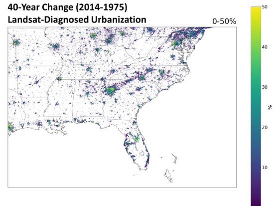
Fig. 1. The 40-year change in urbanization (2014 minus 1975) over the southeast U.S. from the Landsat-based “Built-Up” dataset.
Close examination shows that there has been an increase in manmade structures nearly everywhere that human settlements already existed. I was somewhat surprised to see that these increases are also widespread in Europe, so that we can expect some of the results I summarize below might well extend to other countries.
Quantifying the Urbanization Effect on Surface Air Temperature
I took all hourly-reporting weather stations (ASOS and AWOS), mostly from airports, in the ISD dataset and for all stations having data at least as far back as 1973. I computed the temperature differences at 09 UTC (close to the daily minimum temperature time) between stations no more that 50 km apart, as well as differences in the Landsat Built-Up values (0 to 100). The Built Up datasets are from 4 separate years: 1975, 1990, 2000, and 2014. I used five years of temperature data centered on those four Landsat years for a total of 20 years of August average 09 UTC temperatures to compare to the corresponding four years of urbanization differences. After considerable experimentation, I settled on the four spatial averaging zones shown in Fig. 2 to compute those urbanization differences. This allows a determination of the magnitude of the UHI influence as a function of distance from the thermometer station location.
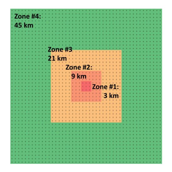
Fig. 2. Averaging zones for Landsat-based “Built-Up” data, nominally at 1 km resolution, for comparison to inter-station temperature differences.
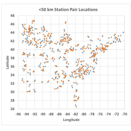
The station pairs used in the analysis are shown in Fig. 3 (sorry for the lack of state boundaries).
When the temperature differences are computed between those station pairs, they can be plotted against the Zone-average differences in urbanization as measured from Landsat. An example for Zone #3 is shown in Fig. 4, where we see the difference in closely spaced station temperatures is indeed related to the difference in Landsat-based urbanization, with some differences in temperature reaching 4 to 5 deg. C (up to 10 deg. F).
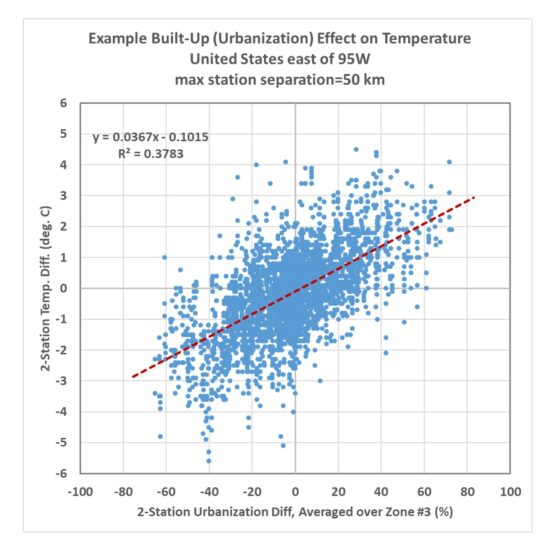
Fig. 4. Twenty years of inter-station temperature differences versus Landsat-based urbanization differences over the eastern United state. Temperature data were the monthly August averages at 09 UTC (close to the time of daily minimum temperature).
The actual algorithm to adjust temperatures uses not just the zone shown in Fig. 4, but all four zones of average Built-Up values in a multiple regression procedure. The resulting coefficients were:
Zone #1: +0.050 deg. C per 10% urbanization difference
Zone #2: +0.061 deg. C per 10% urbanization difference
Zone #3: +0.172 deg. C per 10% urbanization difference
Zone #4: +0.081 deg. C per 10% urbanization difference
The sum of these coefficients is 0.37 deg. C/per 10%, which is essentially the same as the regression coefficient in Fig. 3 for a single zone. The difference is that by using 4 averaging zones together, the correlation is improved somewhat (r=0.67 for the multiple regression), and we also get to see what regions of urbanization have the most influence on the temperatures. From the results above we see all of the averaging zones are important, with Zone 3 contributing the most to explaining the UHI effect on warming, and the 3×3 km zone closest to the thermometer has the last amount of information. Note that I have no information regarding the microclimate right next to the thermometer site (as Anthony uses), so if heat generating equipment was added in the vicinity of the thermometer over the 40 year period 1975-2014, that would not be quantified here and such spurious warming effects will remain in the temperature data even after I have de-urbanized the temperatures.
Application of the Method to Eastern U.S. Temperatures
The resulting regression-based algorithm basically allows one to compute the urban warming effect over time over the last 40-50 years. To the extent that the stations used in the analysis represent all of the eastern U.S., the regression relationship can be applied anywhere in that region, whether there are weather stations there or not.
I applied the method to 269 stations having sufficient data to compute 50-year trends (1973-2022) for August 09 UTC temperatures, and Fig. 5 shows the raw temperature trends versus the de-urbanized temperature trends. When stations in each of the 37 states are averaged together, and the state averages are area-weighted, there is a 40% reduction in the average temperature trend for those 37 states.
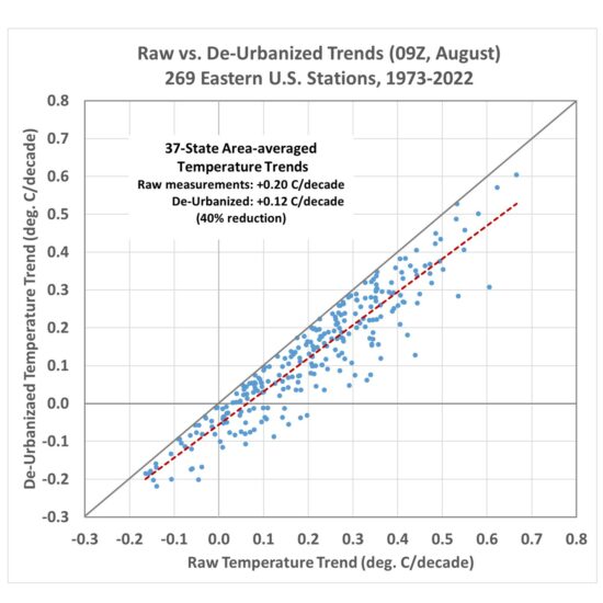
Fig. 5. Raw versus de-urbanized temperature trends across 269 stations in the eastern U.S. for 09 UTC August temperatures (approximately, August daily minimum temperatures).
For the reasons stated above, this might well be an underestimate of the full urbanization effect on eastern U.S. temperature trends.
We can examine the temperature at some individual stations. For example, Figs. 6, 7, 8, and 9 show the raw versus de-urbanized temperatures at Orlando, Indianapolis, Waterloo (IA), and Sault Ste. Marie, (MI). Since I am only dealing with a single month (August) there are no seasonal effects to remove so we can plot actual temperatures rather than temperature anomalies.
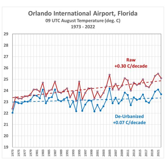
Fig. 6. Average August 09 UTC temperatures, 1973-2022, from raw hourly measurements and after Landsat-based de-urbanization adjustment.
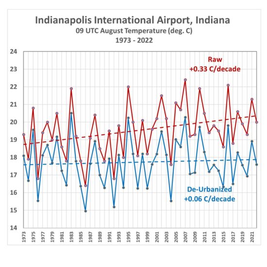
Fig. 7. Indianapolis average August 09 UTC temperatures, 1973-2022, from raw hourly measurements and after Landsat-based de-urbanization adjustment.
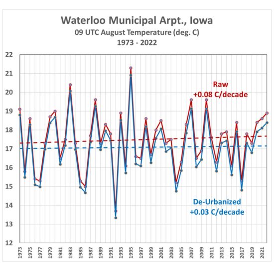
Fig. 8. Waterloo, IA average August 09 UTC temperatures, 1973-2022, from raw hourly measurements and after Landsat-based de-urbanization adjustment.
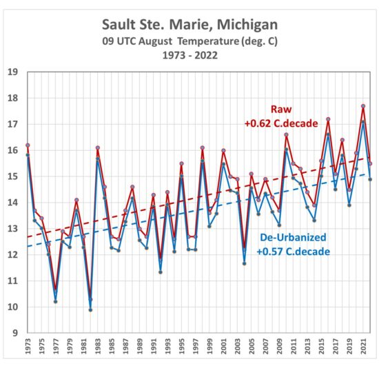
Fig. 9. Sault Ste. Marie, MI, average August 09 UTC temperatures, 1973-2022, from raw hourly measurements and after Landsat-based de-urbanization adjustment.
(As an aside, while I was in the University of Michigan’s Atmospheric and Oceanic Science program, I worked summers at the Sault weather office, and made some of the temperature measurements in Fig. 9 during 1977-1979.)
How Do These Trends Compare to Official NOAA Data?
The statewide-average temperatures from NOAA’s Climate at a Glance website were compared to the corresponding statewide averages computed here. First let’s look at how the raw ISD trends compare to the NOAA-adjusted data (Fig. 10).
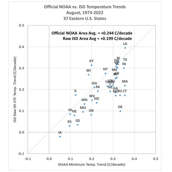
Fig. 10. Statewide-average August temperature trends, 1973-2022, from official NOAA-adjusted data versus the unadjusted hourly temperatures at 09 UTC.
Note the official NOAA temperatures have an average trend higher than the raw ISD data trend (they are mostly independent data sources): +0.244 C/decade vs. +0.199 C/decade. Once the de-urbanization procedure is applied to the individual ISD stations, the results show an average trend fully 50% below that produced by the official NOAA product (Fig. 11).
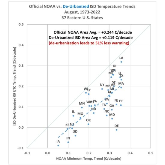
Fig. 11. As in Fig. 10, but after de-urbanization of the ISD 09 UTC temperatures and trends recomputed.
Summary and Conclusions
There is much more I could show, but from the analysis I’ve done so far I believe that the Landsat-based “Built-Up” (urbanization) dataset, which extends back to the 1970s, will be be useful for “de-urbanizing” land-based surface temperature datasets, in the U.S. as well as in other countries. The methodology outlined here is straightforward and the regression statistics are robust (the regression coefficients are all significant, at the 3-sigma level or better).
The urbanization effect on surface temperature trends for August at 09 UTC (near the time of daily minimum temperature) results in a 50% reduction in those trends over the last 50 years. From some preliminary looks I have had at the data from other months and times of day I’d say this will likely be the upper limit of de-urbanization adjustments. So, it is likely that trends in daytime temperature near the time of the daily maximum will not be reduced nearly as much as 50%.
But given the fact that all CMIP6 climate models produce U.S. summer temperature trends greater than the NOAA observations means the discrepancy between climate models and observations is even larger than currently suspected by many of us. John Christy and I believe it is time for a new surface temperature dataset, and the methodology outlined above looks like a viable approach to that end.


Hi there! Someone in my Facebook group shared this website with us so I came to give it a look. I’m definitely enjoying the information. I’m book-marking and will be tweeting this to my followers! Wonderful blog and brilliant design and style.|
Great article.|
When I initially commented I appear to have clicked the -Notify me when new comments are added- checkbox and from now on every time a comment is added I get 4 emails with the exact same comment. There has to be an easy method you are able to remove me from that service? Cheers!|
You made several good points there. I did a search on the subject and found mainly folks will agree with your blog.
I have learn several good stuff here. Definitely value bookmarking for revisiting. I wonder how much attempt you put to make one of these fantastic informative website.
This design is spectacular! You most certainly know how to keep a reader amused. Between your wit and your videos, I was almost moved to start my own blog (well, almost…HaHa!) Great job. I really enjoyed what you had to say, and more than that, how you presented it. Too cool!|
Fantastic website. Lots of helpful info here. I’m sending it to some buddies ans also sharing in delicious. And of course, thank you in your sweat!
You could definitely see your enthusiasm within the work you write. The arena hopes for more passionate writers such as you who are not afraid to say how they believe. Always go after your heart.
Write more, thats all I have to say. Literally, it seems as though you relied on the video to make your point. You definitely know what youre talking about, why throw away your intelligence on just posting videos to your blog when you could be giving us something enlightening to read?|
Asking questions are genuinely fastidious thing if you are not understanding something completely, except this piece of writing provides pleasant understanding even.|
Undeniably believe that which you said. Your favorite reason seemed to be on the internet the simplest thing to be aware of. I say to you, I definitely get annoyed while people think about worries that they just do not know about. You managed to hit the nail upon the top and defined out the whole thing without having side effect , people could take a signal. Will probably be back to get more. Thanks
Why people still make use of to read news papers when in this technological world all is available on web?|
There is definately a lot to learn about this issue. I really like all the points you made.|
Greetings! This is my first comment here so I just wanted to give a quick shout out and tell you I really enjoy reading through your posts. Can you suggest any other blogs/websites/forums that go over the same topics? Appreciate it!|
I love the efforts you have put in this, thanks for all the great posts.
naturally like your website however you have to check the spelling on quite a few of your posts. Several of them are rife with spelling issues and I to find it very bothersome to tell the truth nevertheless I will surely come back again.
Way cool! Some extremely valid points! I appreciate you writing this article and the rest of the site is extremely good.
Hello There. I discovered your blog using msn. This is an extremely neatly written article. I’ll make sure to bookmark it and come back to learn more of your helpful info. Thank you for the post. I will definitely comeback.|
Thanks for sharing your thoughts on meta_keyword. Regards|
If you’re a homeowner looking to get a loan, a secured loan could be a sensible option. Access better rates by using your home as collateral.
I will right away grasp your rss as I can not to find your e-mail subscription hyperlink or e-newsletter service. Do you’ve any? Kindly let me understand so that I may subscribe. Thanks.|
I am regular visitor, how are you everybody? This post posted at this web site is in fact fastidious.|